CPU Scheduling in Operating System
In the previous chapter, we saw how a process, and even individual threads within a process, move through states like Ready and Running, and how context switching allows the operating system to move the CPU between them. What we didn't cover in detail is exactly how the operating system decides which Ready process gets the CPU next, out of possibly many that are waiting at the same time. That decision-making process is called CPU scheduling, and it's one of the most important responsibilities an operating system has, since it directly determines how efficiently the system runs and how responsive it feels to its users.
CPU scheduling becomes necessary because, at any given moment, a computer typically has many more processes wanting to run than it has CPU cores available to run them. Rather than letting processes run in whatever order they happen to arrive, an operating system uses a scheduling algorithm to decide the order and manner in which waiting processes are given access to the CPU, aiming to keep the system efficient and fair at the same time. This chapter walks through five major algorithms, each with a fully solved numerical example, an original Gantt chart, and waiting, turnaround, and response time calculations, followed by practice problems you can attempt on your own.
Why CPU Scheduling Matters
Without any scheduling strategy at all, a computer would simply run one process from start to finish before even considering the next one, exactly like the Batch Operating System covered earlier in this series. This approach wastes enormous amounts of CPU time, since a process very often pauses to wait for input, output, or some other event, during which the CPU would otherwise sit completely idle if no other process was allowed to use it in the meantime. Good CPU scheduling keeps the processor working productively as often as possible, while also making sure no single process is unfairly delayed for an unreasonable length of time.
Common Scheduling Criteria
Before comparing different scheduling algorithms, it helps to understand the specific measures used to judge how well a scheduling algorithm is performing. These criteria appear repeatedly throughout this chapter and in the solved examples that follow.
| Criterion | What It Measures |
|---|---|
| CPU Utilization | How much of the time the CPU is kept busy doing useful work, rather than sitting idle |
| Throughput | The number of processes completed within a given amount of time |
| Turnaround Time | The total time taken from a process arriving in the system to it finishing completely |
| Waiting Time | The total time a process spends waiting in the Ready state before it gets the CPU |
| Response Time | The time from a process arriving until it receives its first response from the CPU |
Turnaround Time, Waiting Time, and Response Time are calculated as follows, and all three are used repeatedly in the solved examples throughout this chapter:
Turnaround Time = Completion Time − Arrival Time
Waiting Time = Turnaround Time − Burst Time
Response Time = Time of First CPU Allocation − Arrival Time
Response Time and Waiting Time are easy to mix up. Waiting Time measures the total time a process spends waiting across its entire life in the system, including any waiting that happens after it has already run once and been preempted. Response Time only measures how long a process waits before it is given the CPU for the very first time — for a non-preemptive algorithm, where a process runs start to finish in one go, the two values end up being identical, but for a preemptive algorithm they are usually different.
Preemptive vs. Non-Preemptive Scheduling
CPU scheduling algorithms are broadly divided into two categories, and this distinction matters throughout the rest of this chapter. In non-preemptive scheduling, once a process is given the CPU, it keeps it until it either finishes completely or voluntarily moves into the Waiting state, such as when it needs to perform an I/O operation. The operating system cannot forcibly take the CPU away from it before then.
In preemptive scheduling, the operating system can interrupt a running process and move it back to the Ready state before it has finished, in order to give the CPU to another process instead, exactly as illustrated by the "Interrupt" transition covered in the previous chapter's process-states diagram. Preemptive scheduling generally improves responsiveness, since a long process cannot indefinitely block shorter, more urgent ones, but it also introduces more frequent context-switching overhead.
Types of CPU Scheduling Algorithms
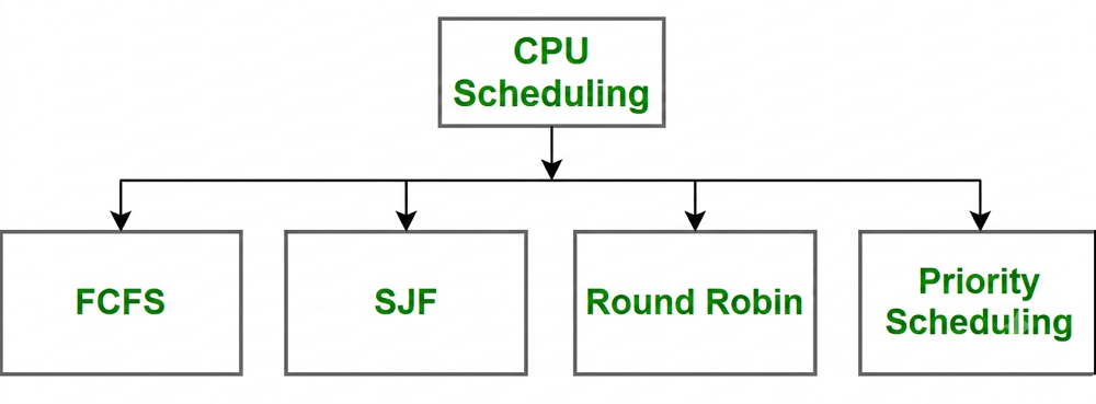
The diagram above shows four of the most commonly studied CPU scheduling algorithms branching out from a central "CPU Scheduling" node: FCFS, SJF, Round Robin, and Priority Scheduling. Each of these algorithms takes a different approach to deciding which Ready process should be given the CPU next, and each comes with its own particular strengths and weaknesses. Alongside these four, this chapter also covers SRTF, the preemptive counterpart to SJF, since it's closely related and commonly studied together with it. The sections below explain each algorithm individually, in the same order shown in the diagram, along with a fully solved numerical example, an original Gantt chart, and response-time calculations for each one.
1. First Come First Serve (FCFS)
First Come First Serve is the simplest possible scheduling algorithm: processes are executed strictly in the order they arrive in the Ready queue, with no consideration given to how long each process will actually take to run. It is a non-preemptive algorithm, meaning once a process starts running, it continues until it finishes completely.
Example: Consider three processes with the following arrival and burst times, where burst time refers to the amount of CPU time a process actually needs to complete.
| Process | Arrival Time | Burst Time |
|---|---|---|
| P1 | 0 | 5 |
| P2 | 1 | 3 |
| P3 | 2 | 8 |
Since FCFS simply follows arrival order, P1 runs first from time 0 to 5, P2 runs next from time 5 to 8, and P3 runs last from time 8 to 16.
Figure 1 (original): FCFS Gantt chart — P1, P2, and P3 run one after another in strict arrival order.
| Process | Completion Time | Turnaround Time | Waiting Time | Response Time |
|---|---|---|---|---|
| P1 | 5 | 5 − 0 = 5 | 5 − 5 = 0 | 0 − 0 = 0 |
| P2 | 8 | 8 − 1 = 7 | 7 − 3 = 4 | 5 − 1 = 4 |
| P3 | 16 | 16 − 2 = 14 | 14 − 8 = 6 | 8 − 2 = 6 |
Average Waiting Time = (0 + 4 + 6) / 3 = 3.33
Average Turnaround Time = (5 + 7 + 14) / 3 = 8.67
Average Response Time = (0 + 4 + 6) / 3 = 3.33
Notice that Response Time and Waiting Time are identical for every process here — this is expected in FCFS, since it's non-preemptive and each process runs in a single, uninterrupted block, so the first (and only) time it gets the CPU is also the point up to which all of its waiting is measured.
The clear drawback of FCFS becomes visible here: P3, despite arriving only slightly after P1, ends up waiting a long time simply because it happened to arrive after two other processes, regardless of how short or long they actually were. This limitation, often called the convoy effect, is exactly what the next algorithm is designed to address.
2. Shortest Job First (SJF)
Shortest Job First selects the Ready process with the smallest burst time to run next, aiming to minimise average waiting time across all processes. This chapter covers the non-preemptive version of SJF, meaning once a process is selected and starts running, it is not interrupted, even if a shorter process arrives afterward.
Example: Using the same three processes as before:
| Process | Arrival Time | Burst Time |
|---|---|---|
| P1 | 0 | 5 |
| P2 | 1 | 3 |
| P3 | 2 | 8 |
At time 0, only P1 has arrived, so it must start running immediately, from time 0 to 5. By the time P1 finishes at time 5, both P2 and P3 have already arrived, so the scheduler compares their burst times and picks P2, the shorter of the two, running it from time 5 to 8. Finally, P3 runs from time 8 to 16.
Figure 2 (original): SJF Gantt chart — in this particular example the schedule happens to match FCFS, since P1 was already running before the shorter P2 arrived.
| Process | Completion Time | Turnaround Time | Waiting Time | Response Time |
|---|---|---|---|---|
| P1 | 5 | 5 − 0 = 5 | 5 − 5 = 0 | 0 − 0 = 0 |
| P2 | 8 | 8 − 1 = 7 | 7 − 3 = 4 | 5 − 1 = 4 |
| P3 | 16 | 16 − 2 = 14 | 14 − 8 = 6 | 8 − 2 = 6 |
In this particular example, the result happens to match FCFS exactly, since P1 had already started before P2 or P3 arrived, leaving the scheduler no real choice at time 0. SJF's real advantage appears more clearly when several short processes are already waiting at the same time a long one is, since SJF will always favour the shorter jobs first in that situation, reducing average waiting time compared to simply following arrival order.
3. Shortest Remaining Time First (SRTF)
Shortest Remaining Time First is the preemptive version of SJF. Instead of committing to a process once it starts, the scheduler compares the remaining burst time of the currently running process against any newly arriving process at every arrival, and switches to the new process immediately if its total burst time is shorter than the running process's remaining time.
Example: Consider these processes:
| Process | Arrival Time | Burst Time |
|---|---|---|
| P1 | 0 | 7 |
| P2 | 2 | 4 |
P1 starts running at time 0, since it's the only process present. At time 2, P2 arrives with a burst time of 4. At this point, P1 has already run for 2 units, leaving 5 units remaining. Since P2's burst time of 4 is shorter than P1's remaining 5, the scheduler preempts P1 and switches to P2. P2 runs to completion from time 2 to 6, since no shorter process arrives to interrupt it. P1 then resumes from time 6, running its remaining 5 units, finishing at time 11.
Figure 3 (original): SRTF Gantt chart — P1 is preempted at time 2 when P2 arrives with a shorter remaining burst, and resumes only after P2 finishes.
| Process | Completion Time | Turnaround Time | Waiting Time | Response Time |
|---|---|---|---|---|
| P1 | 11 | 11 − 0 = 11 | 11 − 7 = 4 | 0 − 0 = 0 |
| P2 | 6 | 6 − 2 = 4 | 4 − 4 = 0 | 2 − 2 = 0 |
Average Waiting Time = (4 + 0) / 2 = 2
Average Response Time = (0 + 0) / 2 = 0
Here the difference between Waiting Time and Response Time becomes clear: P1's Response Time is 0 because it starts running the instant it arrives, but its Waiting Time is 4, because after being preempted at time 2 it still has to wait from time 2 until time 6 — a full 4 units — before it gets the CPU again to finish. Notice how P2, the shorter process, is allowed to finish quickly without waiting behind the longer P1, which is exactly the benefit SRTF offers over plain non-preemptive SJF. The trade-off is the added complexity and context-switching overhead of constantly comparing remaining burst times whenever a new process arrives.
4. Priority Scheduling
Priority Scheduling assigns each process a priority value, and the process with the highest priority, which is usually represented by the lowest priority number, is selected to run next. Like SJF, Priority Scheduling can be implemented as either preemptive or non-preemptive, depending on whether a running process can be interrupted by a newly arrived, higher-priority process.
Example (non-preemptive): Consider three processes arriving at the same time, each with a different priority, where a lower number means higher priority:
| Process | Arrival Time | Burst Time | Priority |
|---|---|---|---|
| P1 | 0 | 4 | 2 |
| P2 | 0 | 3 | 1 |
| P3 | 0 | 5 | 3 |
Since all three arrive at the same time, the scheduler simply picks the process with the best (lowest) priority number first. P2 has priority 1, so it runs first from time 0 to 3. P1 has the next-best priority of 2, running from time 3 to 7. P3, with the lowest priority of 3, runs last, from time 7 to 12.
Figure 4 (original): Priority Scheduling Gantt chart — P2 runs first for having the best (lowest) priority number, followed by P1, then P3.
| Process | Completion Time | Turnaround Time | Waiting Time | Response Time |
|---|---|---|---|---|
| P2 | 3 | 3 − 0 = 3 | 3 − 3 = 0 | 0 − 0 = 0 |
| P1 | 7 | 7 − 0 = 7 | 7 − 4 = 3 | 3 − 0 = 3 |
| P3 | 12 | 12 − 0 = 12 | 12 − 5 = 7 | 7 − 0 = 7 |
Average Waiting Time = (0 + 3 + 7) / 3 = 3.33
Average Response Time = (0 + 3 + 7) / 3 = 3.33
One well-known risk with Priority Scheduling is starvation, where a low-priority process keeps getting delayed indefinitely because higher-priority processes continue arriving ahead of it. A common solution to this problem is a technique called aging, where a process's priority is gradually increased the longer it waits, eventually guaranteeing it will be selected to run.
5. Round Robin (RR)
Round Robin is a preemptive scheduling algorithm designed specifically for time-sharing systems, directly reflecting the Time-Sharing Operating System concept introduced earlier in this series. Each process is given a small, fixed unit of CPU time called a time quantum, and if the process hasn't finished by the time its quantum expires, it is preempted and placed back at the end of the Ready queue, allowing the next process to run.
Example: Consider these processes with a time quantum of 3:
| Process | Arrival Time | Burst Time |
|---|---|---|
| P1 | 0 | 5 |
| P2 | 0 | 4 |
| P3 | 0 | 6 |
With a time quantum of 3, execution proceeds as follows: P1 runs from 0 to 3 (2 units remaining), then P2 runs from 3 to 6 (1 unit remaining), then P3 runs from 6 to 9 (3 units remaining). The queue then cycles back: P1 runs from 9 to 11 and finishes, P2 runs from 11 to 12 and finishes, and P3 runs from 12 to 15 and finishes.
Figure 5 (original): Round Robin Gantt chart with time quantum 3 — every process gets a repeated, bounded turn instead of running to completion in one block.
| Process | Completion Time | Turnaround Time | Waiting Time | Response Time |
|---|---|---|---|---|
| P1 | 11 | 11 − 0 = 11 | 11 − 5 = 6 | 0 − 0 = 0 |
| P2 | 12 | 12 − 0 = 12 | 12 − 4 = 8 | 3 − 0 = 3 |
| P3 | 15 | 15 − 0 = 15 | 15 − 6 = 9 | 6 − 0 = 6 |
Average Waiting Time = (6 + 8 + 9) / 3 = 7.67
Average Response Time = (0 + 3 + 6) / 3 = 3
Round Robin's Response Time values are noticeably better than its Waiting Time values, and this is exactly why Round Robin feels so responsive in interactive systems — every process is guaranteed to get its first turn on the CPU quickly, even though it may still have to wait through several more rounds before it fully finishes. Round Robin's biggest strength is fairness — every process gets a guaranteed, regular turn on the CPU. Its main trade-off is that choosing the time quantum matters a great deal: too large a quantum and Round Robin starts behaving like FCFS, while too small a quantum causes excessive context-switching overhead, reducing overall CPU efficiency.
Comparison of CPU Scheduling Algorithms
| Algorithm | Preemptive? | Best Suited For | Main Drawback |
|---|---|---|---|
| FCFS | No | Simple batch-style systems | Convoy effect, poor average waiting time |
| SJF | No | Systems where burst times are known in advance | Can starve longer processes |
| SRTF | Yes | Systems needing quick response to short jobs | High context-switching overhead |
| Priority Scheduling | Either | Systems where some tasks are genuinely more urgent | Starvation of low-priority processes without aging |
| Round Robin | Yes | Interactive, time-sharing systems | Performance heavily depends on time quantum size |
Practice Problems
The best way to get comfortable with CPU scheduling is to work through a few problems yourself before checking the answer. Try sketching your own Gantt chart on paper for each of the following, then use the formulas from earlier in this chapter to calculate the average waiting, turnaround, and response times. Expand each answer only after you've attempted the problem.
Practice Problem 1 — FCFS
| Process | Arrival Time | Burst Time |
|---|---|---|
| P1 | 0 | 6 |
| P2 | 2 | 2 |
| P3 | 4 | 4 |
Schedule these three processes using FCFS and calculate the average waiting time and average turnaround time.
Show Answer
Waiting times: P1 = 0, P2 = 4, P3 = 4. Average Waiting Time = 2.67.
Turnaround times: P1 = 6, P2 = 6, P3 = 8. Average Turnaround Time = 6.67.
Practice Problem 2 — SJF (Non-Preemptive)
| Process | Arrival Time | Burst Time |
|---|---|---|
| P1 | 0 | 8 |
| P2 | 0 | 4 |
| P3 | 0 | 2 |
| P4 | 0 | 6 |
All four processes arrive at the same time. Schedule them using non-preemptive SJF and calculate the average waiting time.
Show Answer
Waiting times: P3 = 0, P2 = 2, P4 = 6, P1 = 12. Average Waiting Time = 5.
Practice Problem 3 — Priority Scheduling (Preemptive)
| Process | Arrival Time | Burst Time | Priority (lower = higher priority) |
|---|---|---|---|
| P1 | 0 | 6 | 3 |
| P2 | 1 | 2 | 1 |
| P3 | 2 | 4 | 2 |
This time, scheduling is preemptive: a newly arriving process interrupts the current one immediately if its priority number is lower. Work out the Gantt chart and the completion time of each process.
Show Answer
Completion times: P2 = 3, P3 = 7, P1 = 12.
Practice Problem 4 — Round Robin (Time Quantum = 2)
| Process | Arrival Time | Burst Time |
|---|---|---|
| P1 | 0 | 5 |
| P2 | 0 | 3 |
Schedule these two processes with a time quantum of 2 and calculate each process's response time.
Show Answer
Response times: P1 = 0 (starts immediately at time 0), P2 = 2 (first runs at time 2).
Completion times: P2 = 7, P1 = 8.
Best Practices While Learning CPU Scheduling
- Always calculate Turnaround Time, Waiting Time, and Response Time using the three formulas shown at the start of this chapter, since nearly every numerical question relies on them.
- Draw a simple Gantt chart, a timeline showing which process runs during which interval, before attempting to fill in a table of completion times — it makes preemptive examples like SRTF and Round Robin far easier to track, and the original charts throughout this chapter show exactly how to lay one out.
- Keep the preemptive-versus-non-preemptive distinction in mind for every algorithm, since it directly affects how a newly arriving process is handled.
- Attempt the practice problems above before revealing the answers — working through the Gantt chart yourself is what actually builds the skill, not just reading a solved example.
- Revisit this chapter before studying Process Synchronization next, since scheduling and synchronization are closely connected whenever multiple processes share resources.
Common Mistakes Beginners Make
| Mistake | Correct Practice |
|---|---|
| Forgetting that a process must have already arrived before it can be considered by the scheduler. | Always check each process's arrival time before assuming it's available to run at a given moment. |
| Applying non-preemptive SJF logic to an SRTF question, or vice versa. | Confirm whether a question is preemptive before deciding if a running process can be interrupted by a new arrival. |
| Assuming a smaller time quantum in Round Robin is always better. | Remember that a very small quantum increases context-switching overhead, while a very large one behaves like FCFS. |
| Confusing Response Time with Waiting Time in preemptive algorithms. | Remember that Response Time only measures the wait until the first CPU allocation, while Waiting Time adds up all the time spent waiting across every preemption. |
Frequently Asked Interview Questions
-
What is CPU scheduling?
CPU scheduling is the process by which the operating system decides which of the Ready processes should be given access to the CPU next. -
What is the difference between preemptive and non-preemptive scheduling?
In non-preemptive scheduling, a running process keeps the CPU until it finishes or voluntarily waits, while in preemptive scheduling, the operating system can interrupt a running process to give the CPU to another one. -
What is the convoy effect in FCFS scheduling?
The convoy effect occurs when a short process gets stuck waiting behind a long process simply because it arrived later, increasing average waiting time significantly. -
What is the difference between SJF and SRTF?
SJF is non-preemptive and commits to a process once it starts, while SRTF is the preemptive version, which can interrupt a running process if a newly arrived process has a shorter remaining burst time. -
What is the difference between Waiting Time and Response Time?
Waiting Time is the total time a process spends waiting in the Ready state across its entire life in the system, while Response Time only measures the time until the process receives the CPU for the first time. -
What is starvation in Priority Scheduling, and how can it be solved?
Starvation happens when a low-priority process is repeatedly delayed by higher-priority processes; it can be solved using aging, which gradually increases a waiting process's priority over time. -
Why is time quantum size important in Round Robin scheduling?
A very small time quantum causes excessive context-switching overhead, while a very large time quantum makes Round Robin behave similarly to FCFS, so choosing an appropriate size is important for good performance. -
How is Waiting Time calculated?
Waiting Time is calculated by subtracting the Burst Time from the Turnaround Time, where Turnaround Time itself is the Completion Time minus the Arrival Time.
Summary
CPU scheduling determines exactly how efficiently and fairly a system shares its processor among competing processes. We looked at the key scheduling criteria used to judge an algorithm's performance, including the often-confused pair of Waiting Time and Response Time, and the important distinction between preemptive and non-preemptive scheduling. We then worked through fully solved numerical examples, each with an original Gantt chart, for five major algorithms: FCFS, SJF, SRTF, Priority Scheduling, and Round Robin, comparing their strengths, weaknesses, and best-suited use cases along the way.
Finally, the four practice problems gave you a chance to apply everything from this chapter yourself, from a straightforward FCFS schedule to a preemptive Priority Scheduling scenario with multiple mid-execution interruptions. With a solid understanding of how the CPU is scheduled among processes, you're now ready to move into Process Synchronization, which addresses what happens when multiple processes or threads need to safely share data and resources while all competing for the same CPU.